- Color
- Usage
Usage
The Color module is very powerful - offering capabilities surpassing most other software - yet it is simple to use.
The primary goal that the Color module was designed to accomplish, is achieving a good colour balance that accurately describes the colour ratios that were recorded. In accomplishing that goal, the Color module goes further than other software by offering a way to negate the adverse effects of non-linear dynamic range manipulations on the data (thanks to Tracking data mining). In simple terms, this means that colouring can be reproduced (and compared!) in a consistent manner regardless of how bright or dim a part of the scene is shown.
A second unique feature of StarTools, is its ability to process luminance (detail) and chrominance (colour) separately, yet simultaneously. This means that any decisions you make affecting your detail does not affect the colouring of said detail, and vice-versa. This ability further allows you to remap colour channels (aka "tone mapping") for narrowband data, without having to start over with your detail processing. This lets you try out many different popular color schemes at the click of a button.
Launching the Color module
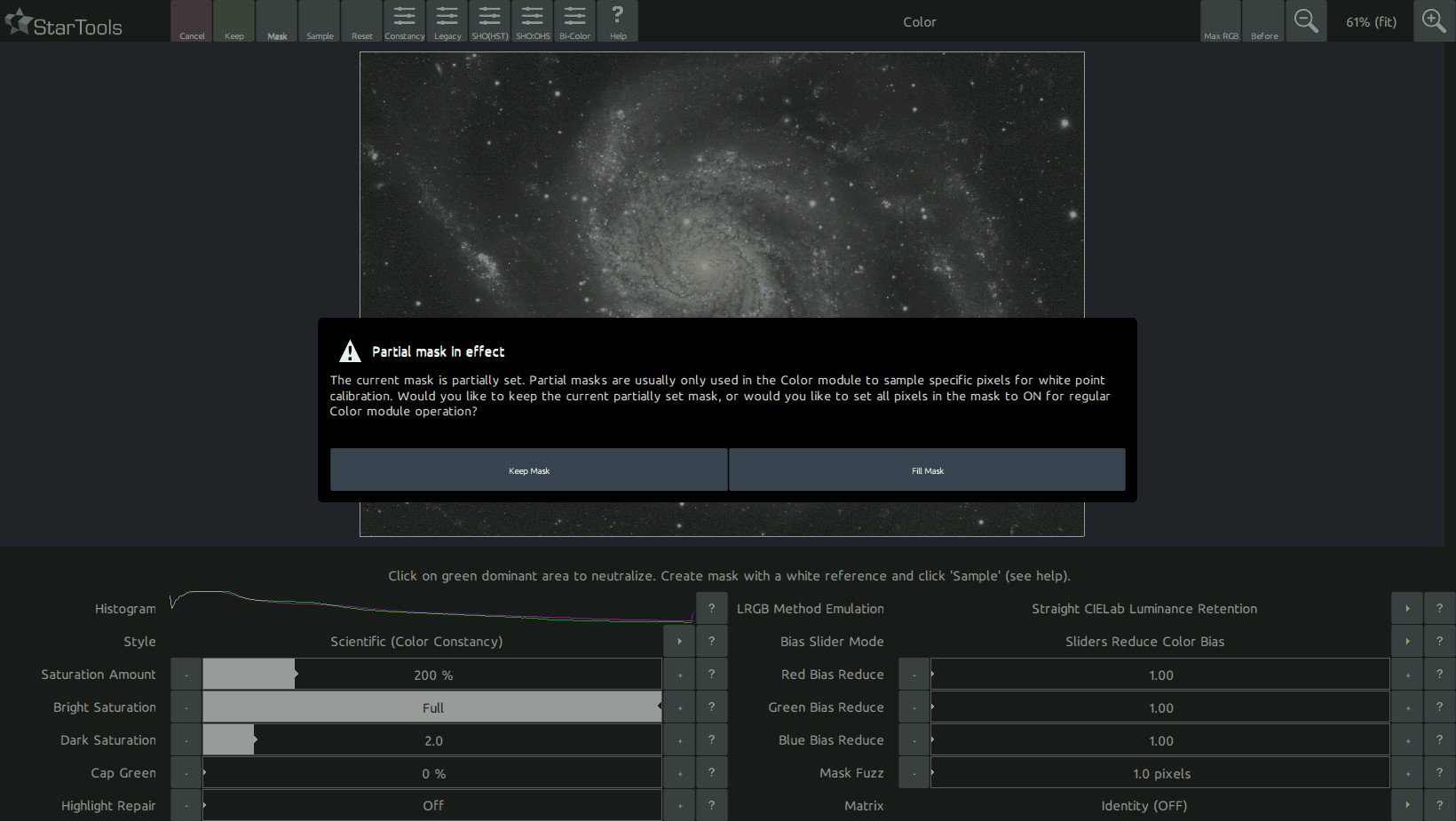
Upon launch, the colour module blinks the mask three times in the familiar way. If a full mask is not set, the Color modules allows you to set it now, as colour balancing is typically applied to the full image (requiring a full mask).
In addition to blinking the mask, the Color module also analyses the image and sets the 'Red, Green and Blue Increase/Reduce' parameters to a value which it deems the most appropriate for your image. This behaviour is identical to manually clicking the 'Sample' button where the whole image is sampled.
In cases where the image contains aberrant colour information in the highlights, for example due to chromatic aberration or slight channel misalignment/discrepancies, then this initial colour balance may be significantly incorrect and may need further correction. The aberrant colour information in the highlights itself, can be repaired using the 'Highlight Repair' parameter.
Setting a colour balance
The 'Red, Green and Blue Increase/Reduce' parameters are the most important settings in the Color module. They directly determine the colour balance in your image. Their operation is intuitive; is there too much red in your image? Then increase the 'Red Bias Reduce' value. Too little red in your image? Reduce the 'Red Bias Reduce' value.
If you would rather operate on these values in terms of Bias Increase, then simply switch the 'Bias Slider Mode' setting to 'Sliders Increase Color Bias'. The values are now represented in terms of relative increases, rather than decreases. Switching between these two modes you can see that, for example, a Red Bias Reduce of 8.00 is the same as a Green and Blue Bias Increase of 8.00. This should make intuitive sense; a relative decrease of red makes blue and green more prevalent and vice versa.
Color balancing techniques
Now that we know how to change the colour balance, how do we know what to actually set it to?
The goal of color balancing in astrophotography, is achieving an accurate representation of emissions, temperatures and processes. A visual spectrum dataset should show emissions where they occur in the blend of colours they occur in. A narrowband dataset, equally, should be rendered as an accurate representation of the relative ratio of emissions (but not necessarily with the color they correspond to the wavelength they appear at in the visual spectrum). So, in all cases, whether your dataset is a visual spectrum dataset or a narrowband dataset, it should let your viewers allow to compare different areas in your image and accurately determine what emissions are dominant, where.
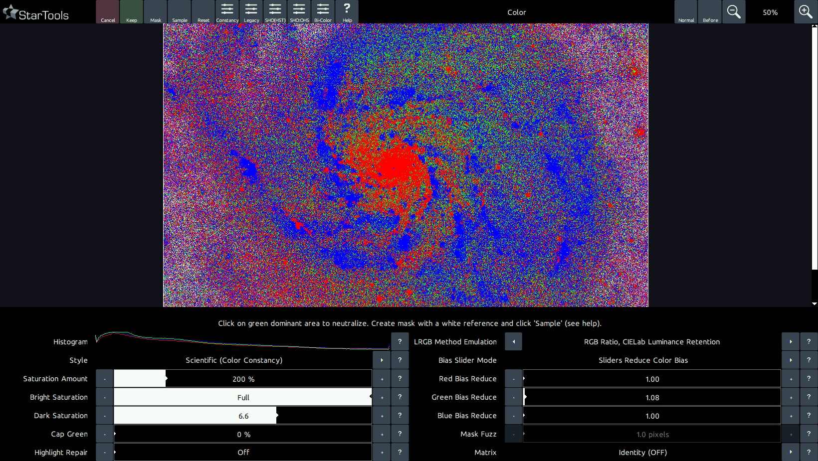
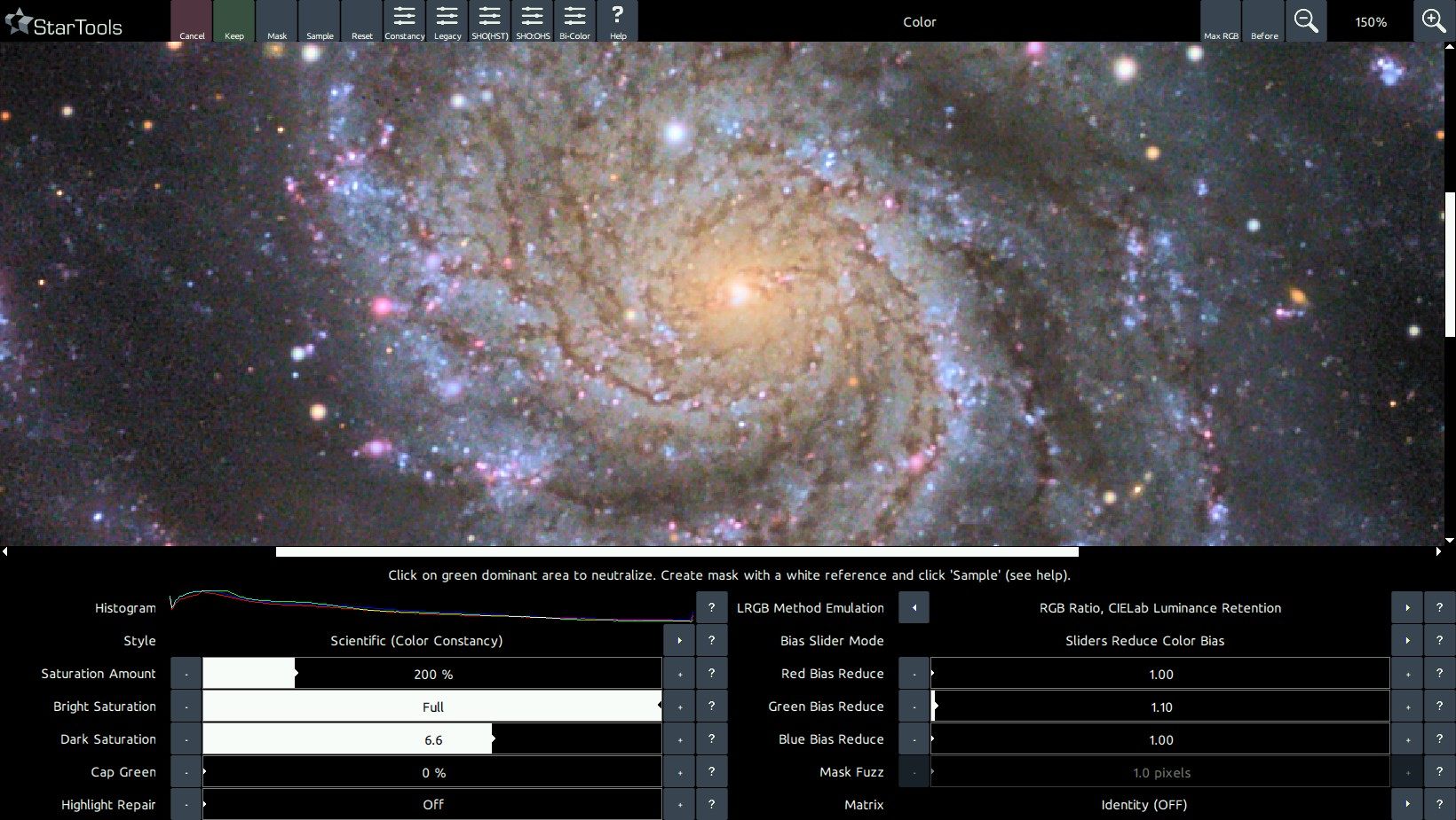
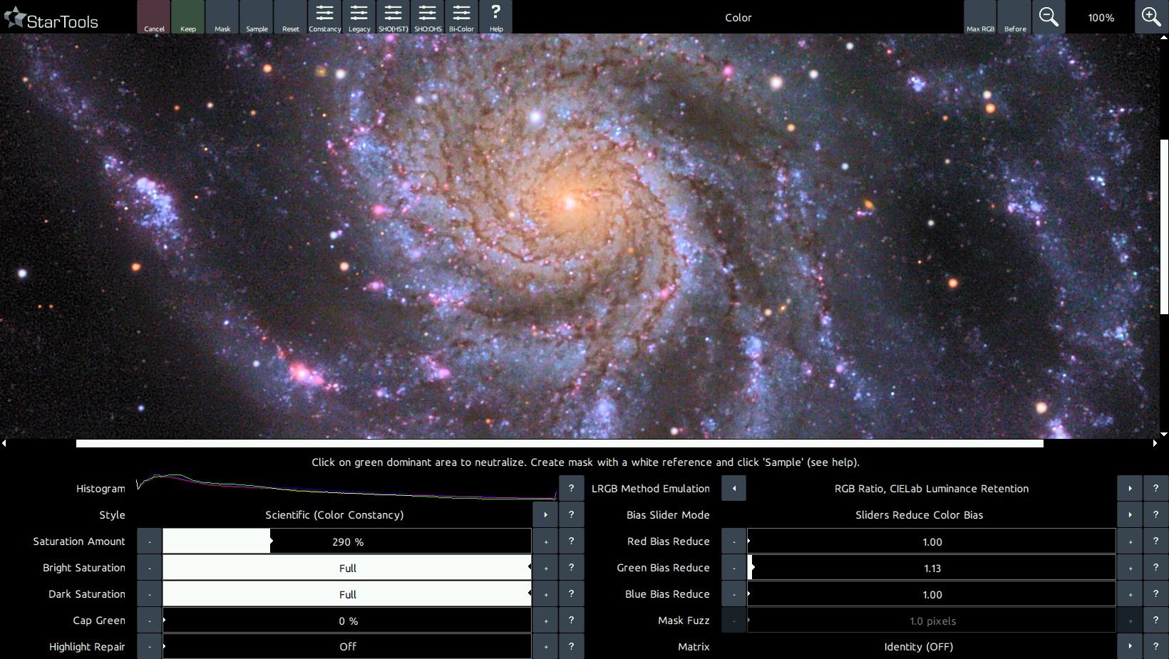
There are a great number of tools and techniques that can be applied in StarTools that let you home in on a good colour balance. Before delving into them, It is highly recommended to switch the 'Style' parameter to 'Scientific (Color Constancy)' during colour balancing, even if that is not the preferred style of rendering the colour of the end result, this is because the Color Constancy feature makes it much easier to colour balance by eye in some instances due to its ability to show continuous, constant colour throughout the image. Once a satisfactory colour balance is achieved you should, of course, feel free to switch to any alternative style of colour rendering.
White point reference by mask sampling
Upon launch the Color module samples whatever mask is set (note also that the set mask also ensures the Color module only applies any changes to the masked-in pixels!) and sets the 'Red, Green and Blue Increase/Reduce' parameters accordingly.
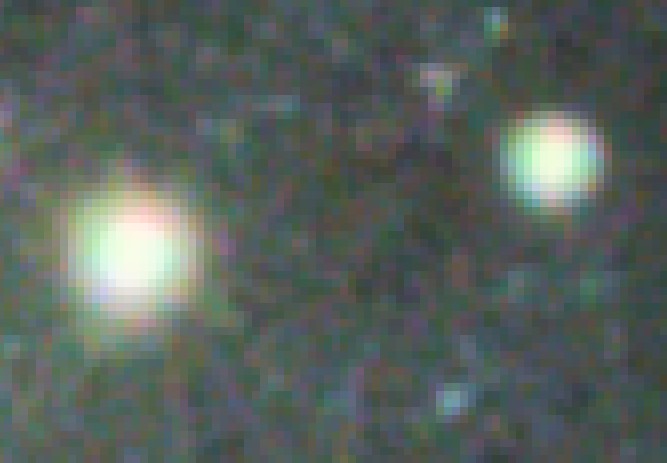
We can use this same behaviour to sample larger parts of the image that we know should be white. This method mostly exploits the fact that stars come in all sorts of sizes and temperatures (and thus colours!) and that this distribution is usually completely random in a wide enough field. Indeed, the Milky Way is named as such because the average color of all its stars is perceived as a milky white. Therefore if we sample a large enough population of stars, we should find the average star color to be - likewise - white .
We can accomplish that in two ways; we either sample all stars (but only stars!) in a wide enough field, or we sample a whole galaxy that happens to be in the image (note that the galaxy must be of a certain type to be a good candidate and be reasonably close - preferably a barred spiral galaxy much like our own Milkyway).
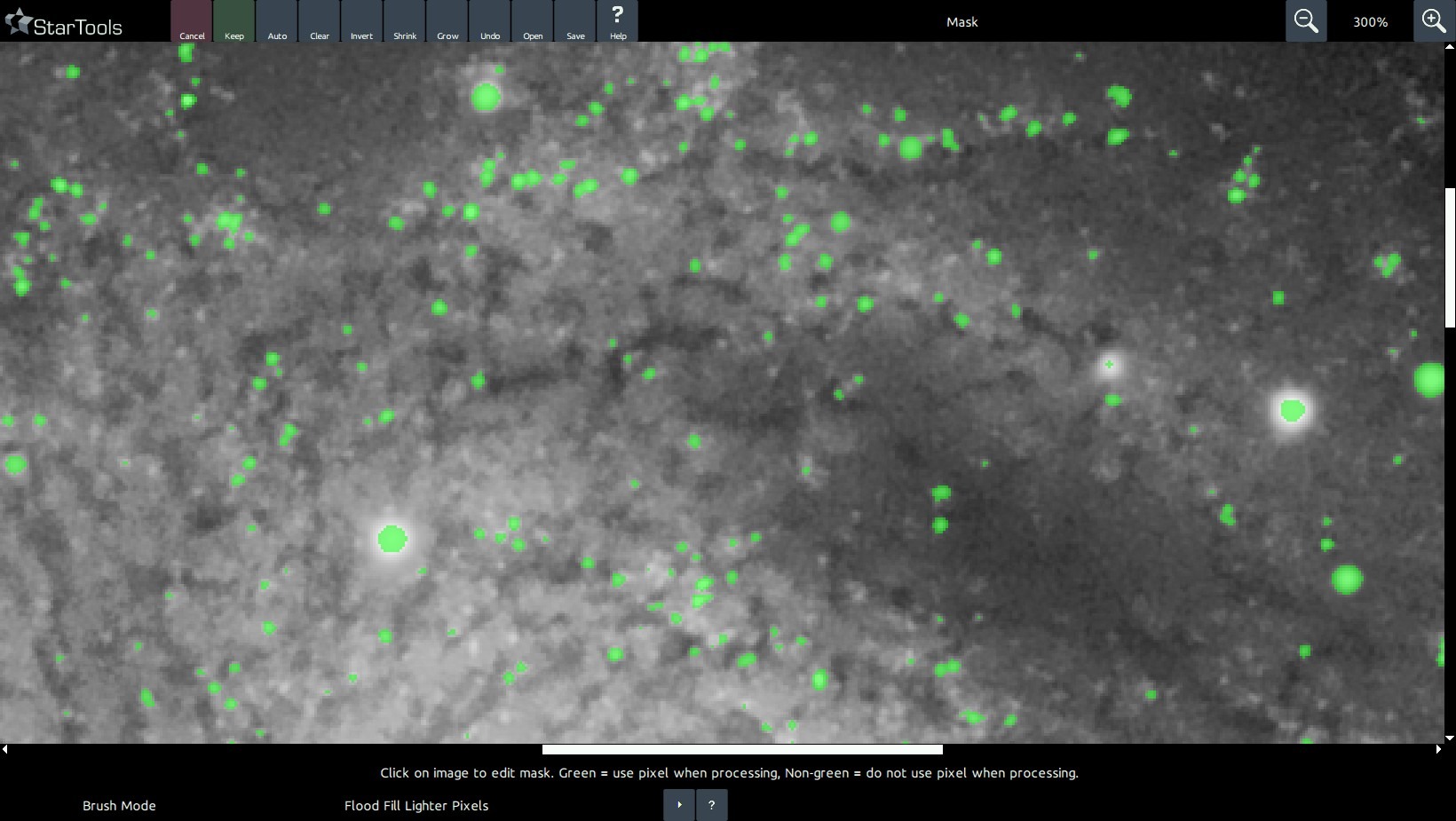
Whichever you choose, we need to create a mask, so we launch the Mask editor. Here we can use the Auto feature to select a suitable selection of stars, or we can us the Flood Fill Brighter or Lassoo tool to select a galaxy. Once selected, return to the Color module and click Sample. StarTools will now determine the correct 'Red, Green and Blue Increase/Reduce' parameters to match the white reference pixels in the mask so that they come out neutral.
To apply the new colour balance to the whole image, launch the Mask editor once more and click Clear, then click Invert to select the whole image. Upon return to the Color module, the whole image will now be balanced by the Red, Green and Blue bias values we determined earlier with just the white reference pixels selected.
White balancing in MaxRGB mode
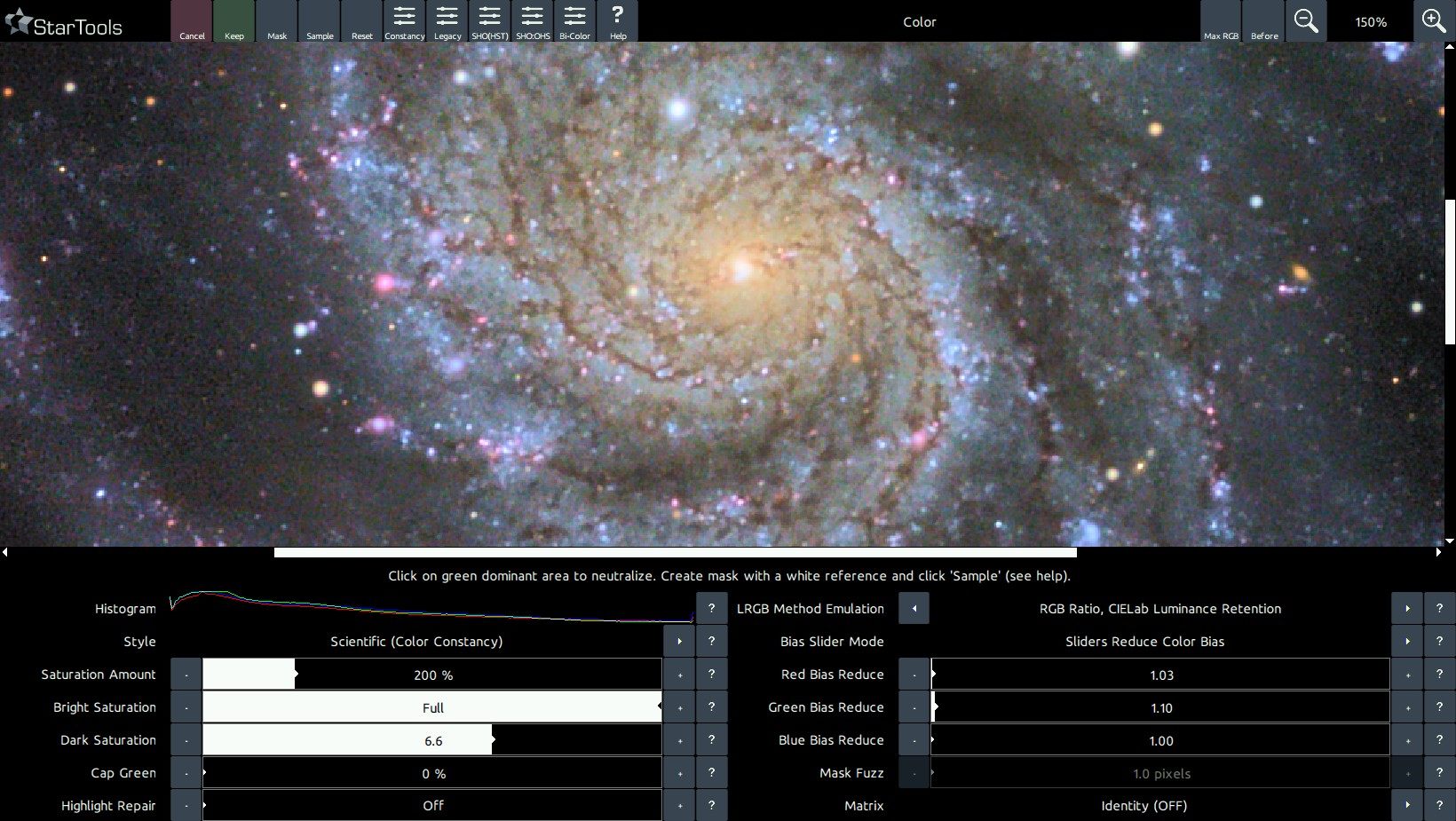
StarTools comes with a unique colour balancing aid called MaxRGB. This mode of colour balancing is exceptionally useful if trying to colour balance by eye, but the user suffers from colour blindness or uses a screen that is not colour calibrated very well. The mode can be switched on or off by clicking on the MaxRGB mode button in the top right corner.
The MaxRGB aid allows you to view which channel is dominant per-pixel. If a pixel is mostly red, that pixel is shown red, if a pixel is mostly green, that pixel is shown green, and if a pixel is mostly blue, that pixel is shown blue.
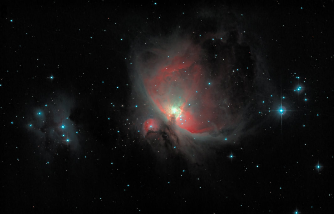
By cross referencing the normal image with the MaxRGB image, it is possible to find deficiencies in the colour balance. For example, the colour green is very rarely dominant in space (with the exception of highly dominant OIII emission areas in, for example the Trapezium in M42).
Therefore, if we see large areas of green, we know that we have too much green in our image and we should adjust the bias accordingly. Similarly if we have too much red or blue in our image, the MaxRGB mode will show many more red than blue pixels in areas that should show an even amount (for example the background). Again we then know we should adjust red or green accordingly.
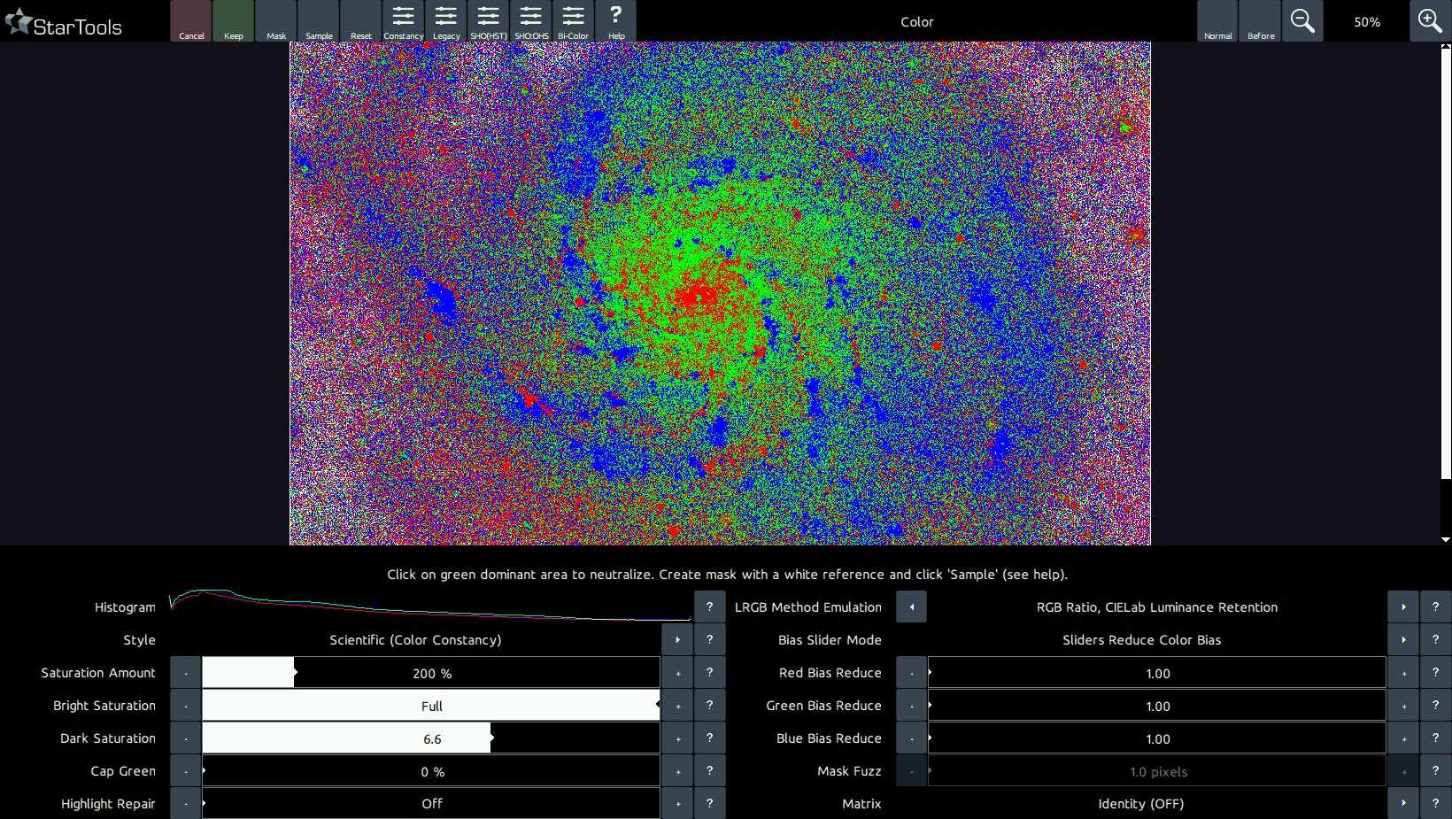
Clicking on an area to neutralise green
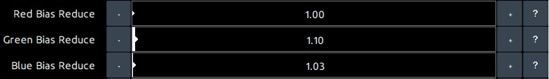
A convenient way to eliminate green dominance is to simply click on an area. The Color module with adjust the 'Green Bias Reduce' or 'Green Bias Increase' in response so that any green dominance in that area is neutralised.
White balancing by known features and processes

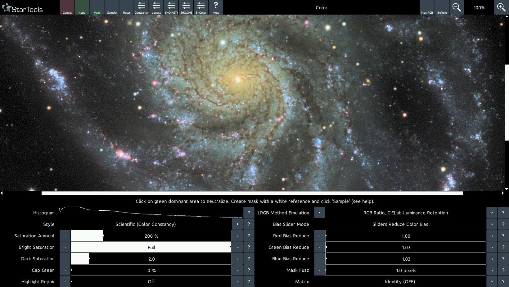
StarTools' Color Constancy feature makes it much easier to see colours and spot processes, interactions, emissions and chemical composition in objects. In fact, the Color Constancy feature makes colouring comparable between different exposure lengths and different gear. This allows for the user to start spotting colours repeating in different features of comparable objects. Such features are, for example, the yellow cores of galaxies (due to the relative over representation of older stars as a result of gas depletion), the bluer outer rims of galaxies (due to the relative over representation of bright blue young stars as a result of the abundance of gas) and the pink/purplish HII area 'blobs' in their discs. Red/brown (white light filtered by dust) dust lanes complement a typical galaxy's rendering.
Similarly, HII areas in our own galaxy (e.g. most nebulae), while in StarTools Color Constancy Style mode, display the exact same colour signature found in the galaxies; a pink/purple as a result of predominantly deep red Hydrogen-alpha emissions mixed with much weaker blue/green
emissions of Hydrogen-beta and Oxygen-III emissions and (more dominantly) reflected blue star light from bright young blue giants who are often born in these areas, and shape the gas around them.
Dusty areas where the bright blue giants have 'boiled away' the Hydrogen through radiation pressure (for example the Pleiades) reflect the blue star light of any surviving stars, becoming distinctly blue reflection nebulae. Sometimes gradients can be spotted where (gas-rich) purple gives away to (gas-poor) blue (for example the Rosette core) as this process is caught in the act.
Diffraction spikes, while artefacts, also can be of great help when calibrating colours; the "rainbow" patterns (though skewed by the dominant colour of the star whose light is being diffracted) should show a nice continuum of colouring.
Finally, star temperatures, in a wide enough field, should be evenly distributed; the amount of red, orange, yellow, white and blue stars should be roughly equal. If any of these colors are missing or are over-represented we know the colour balance is off.
Colour balancing of data that was filtered by a light pollution filter
Colour balancing of data that was filtered by a light pollution filter is fundamentally impossible; narrow (or wider) bands of the spectrum are missing and no amount of colour balancing is going to bring them back and achieve proper colouring. A typical filtered data set will show a distinct lack in yellow and some green when properly colour balanced. It's by no means the end of the world - it's just something to be mindful of.
Correct colouring may be achieved however by shooting deep luminance data with light pollution filter in place, while shooting colour data without filter in place, after which both are processed separately and finally combined. Colour data is much more forgiving in terms of quality of signal and noise; the human eye is much more sensitive to noise in the luminance data that it is in the colour data. By making clever use of that fact and performing some trivial light pollution removal in Wipe, the best of both worlds can be achieved.
OSC (One-Shot-Color) instruments
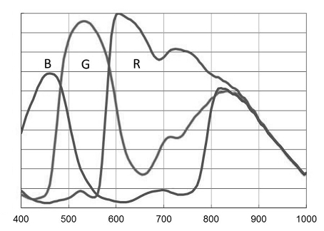
Many modern OSC cameras have a spectrum response that increases in sensitivity across all channels beyond the visual spectrum red cut-off (the human eye can detect red wavelengths up until around 700nm). This is a feature that allows these cameras pick up detail beyond the visual spectrum (for example for use with narrowband filters or for recording infrared detail).
However, imaging with these instruments without a suitable IR/UV filter (also known as a "luminance filter") in place, will cause these extra-visual spectrum wavelengths to accumulate in the visual spectrum channels. This can significantly impact the "correct" (in terms of visual spectrum) colouring of your image. Just as a light pollution filter makes it fundamentally impossible to white-balance back the missing signal, so too does imaging with extended spectrum response make it impossible to white-balance the superfluous signal away.
Hallmarks of datasets that have been acquired with such instruments, without a suitable IR/UV filter in place, is a distinct yellow cast that is hard (impossible) to get rid of, due to a strong green response coming back in combined with extended red channel tail.
The solution is to image with a suitable IR/UV filter in place that cuts-off the extended spectrum response before those channels increase in sensitivity again. The needed IR/UV filter will vary per OSC. Consult the respective manufacturers' spectral graphs to find the correct match for your OSC.
Tweaking your colors
Once you have achieved a color balance you are happy with, the StarTools Color module offers a great number of ways to change the presentation of your colours.
Style
The parameter with the biggest impact is the 'Style' parameter. StarTools is renowned for its Color Constancy feature, rendering colours in objects regardless of how the luminance data was stretched, the reasoning being that colours in outer space don't magically change depending on how we stretch our image. Other software sadly lets the user stretch the colour information along with the luminance information, warping, distorting and destroying hue and saturation in the process. The 'Scientific (Color Constancy)' setting for Style undoes these distortions using Tracking information, arriving at the colours as recorded.
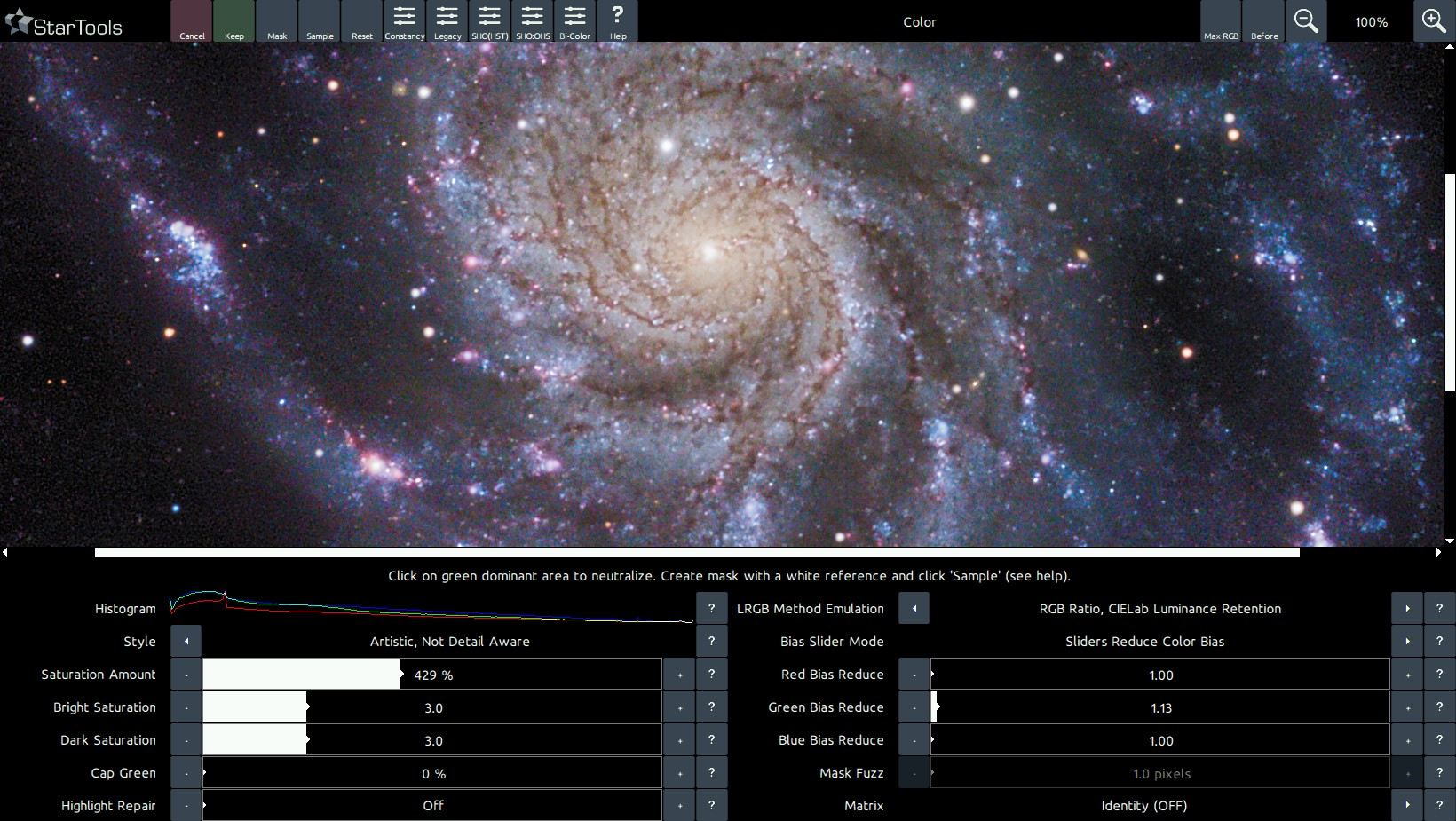
To emulate the way other software renders colours, two other settings are available for the 'Style' parameter. These settings are "Artistic, Detail Aware" and "Artistic, Not Detail Aware". The former still uses some Tracking information to better recover colours in areas whose dynamic range was optimised locally, while the latter does not compensate for any distortions whatsoever.
LRGB Method Emulation
The 'LRGB Method Emulation' parameter allows you to emulate a number of colour compositing methods that have been invented over the years. Even if you acquired data with an OSC or DSLR, you will still be able to use these compositing methods; the Color module will generate synthetic luminance from your RGB on the fly and re-composite the image in your desired compositing style.
The difference in colouring can be subtle or more pronounced. Much depends on the data and the method chosen.
- 'Straight CIELab Luminance Retention' manipulates all colours in a psychovisually optimal way in CIELab space, introducing colour without affecting apparent brightness.
- 'RGB Ratio, CIELab Luminance Retention' uses a method first proposed by Till Credner of the Max-Planck-Institut and subsequently rediscovered by Paul Kanevsky, using RGB ratios multiplied by luminance in order to better preserve star colour. Luminance retention in CIELab color space is applied afterwards.
- '50/50 Layering, CIELab Luminance Retention' uses a method proposed by Robert Gendler, where luminance is layered on top of the colour information with a 50% opacity. Luminance retention in CIELab color space is applied afterwards. The inherent loss of 50% in saturation is compensated for, for your convenience, in order to allow for easier comparison with other methods.
- 'RGB Ratio' uses a method first proposed by Till Credner of the Max-Planck-Institut and subsequently rediscovered by Paul Kanevsky, using RGB ratios multiplied by luminance in order to better preserve star colour. No further luminance retention is attempted.
- '50/50 Layering, CIELab Luminance Retention' uses a method proposed by Robert Gendler, where luminance is layered on top of the colour information with a 50% opacity. No further luminance retention is attempted. The inherent loss of 50% in saturation is compensated for, for your convenience, in order to allow for easier comparison with other methods.
When processing a complex composite that carries a luminance signal that is substantially decoupled from the chrominance signal (for example importing H-alpha as luminance and a visual spectrum dataset as red, green and blue via the Compose module), then the 'RGB Ratio, CIELab Luminance Retention' will typically do a superior job accommodating the greater disparities in luminance and how this affect final colouring.
Finally, please note that the LRGB Emulation Method feature is only available when Tracking is engaged.
Saturation
The 'Saturation' parameter allows colours to be rendered more, or less vividly, whereby the 'Bright Saturation' parameter and 'Dark Saturation' parameter control how much colour and saturation is introduced in the highlights and shadows respectively. It is important to note that introducing colour in the shadows may exacerbate colour noise, though Tracking will make sure any such noise exacerbations are recorded and dealt with during the final denoising stage.
Cap Green
The 'Cap Green' parameter, finally, removes spurious green pixels if needed, reasoning that green dominant colours in outer space are rare and must therefore be caused by noise. Use of this feature should be considered a last resort if colour balancing does not yield adequate results and the green noise is severe. The final denoising stage should, thanks to Tracking data mining, pin pointed the green channel noise already and should be able to adequately mitigate it.
Matrix correction and on-the-fly channel remapping
The Color module comes with a vast number of camera color correction matrices for various DSLR manufacturers (Canon, Nikon, Sony, Olympus, Pentax and more), as well as a vast number of channel blend remappings (aka "tone mapping") for narrowband dataset (e.g. HST/SHO or bi-color duoband/quadband filter data).
Uniquely, thanks to the signal evolution Tracking engine, color calibration is preferably performed towards the end of your processing workflow. This allows you to switch color rendering at the very last moment at the click of a button without having to re-composite and re-process, while also allowing you to use cleaner, non-whitebalanced, non-matrix corrected data for your luminance component, aiding signal fidelity.
Camera Matrix correction is performed towards the end of your processing workflow on your chrominance data only, rather than in the RAW converter during stacking. This helps improve luminance (detail) signal, by not contaminating it with cross-channel camera-space RGB and XYZ-space manipulations.
The matrix or channel blend/mapping is selected using the 'Matrix' parameter. Please note that the available options under this parameter are dependent on the type of dataset you imported. Please use the Compose module to import any narrowband data separately.
Presets
As in most modules in StarTools, a number of presets are available to quickly dial in useful starting points.
- 'Constancy' sets the default Color Constancy mode and is the recommended mode for diagnostics and color balancing in.
- 'Legacy' switches to a color rendition for visual spectrum datasets that is closest to what legacy software (e.g. software without signal evolution Tracking) would produce. This will mimic the way such software (incorrectly) desturates highlights and causes hue shifts.
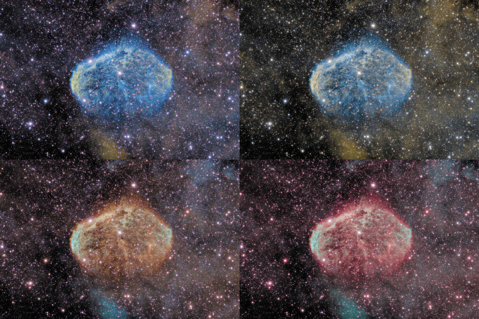
- 'SHO(HST)' dials in settings that are a good starting point for datasets that were imported as S-II, H-alpha and O-III for red, green and blue respectively (also known as the 'SHO, 'SOH:RGB', 'HST' or 'Hubble' palette). This standard way of importing datasets and mapping the 3 bands to the 3 channels in this way (via the Compose module), allows for further channel blends and remapping via the 'Matrix' parameter. Please note the specific blend's parameters/factors under the 'Matrix' parameter. This preset also greatly reduces the green bias to minimise green, while attempting to bring out the popular golden hues.
- 'SHO:OHS' is similar to the 'SHO(HST)' preset, except that it further remaps a SHO-imported dataset to a channel blend that is predominantly mapped as OHS:RGB instead. Renditions typically yield a pleasing "glowing ice-on-fire" effect.
- 'Bi-Color' assumes a dataset was imported as HOO:RGB, that is Ha-alpha imported as red, and O-III (sometimes also incorporating H-beta) imported as green and also blue. This yields the popular red/cyan bi-color renderings that are so effective at showing dual emission dominance. This preset is also particularly useful and popular for people who use a duo-band filter (aka as a tri-band or quad-band filter) with an OSC or DSLR.
You may also be interested in...
- L. B., United States (under Testimonials)
I'm relatively new to image processing and just wanted to say how straight forward and powerful StarTools is.
- HDR: Automated Local Dynamic Range Optimization (under Features & Documentation)
The HDR (High Dynamic Range) module optimises local dynamic range, recovering small to medium detail from your image.
- Usage (under Shrink)
The 'AutoMask' button launches a popup with access to two quick ways of creating a star mask.
- Parameters (under Usage)
The 'Color Taming' parameter forces stars to progressively adopt the colouring of their surroundings, like "chameleons".
- Creating a suitable star mask (under Usage)
This time set 'Old Mask' to 'Add New To Old' to add the newly generated mask to the mask we already have.